Demystifying ‘Confusion Matrix’ Confusion
If you are Confused about Confusion Matrix, then I hope this post may help you understand it! Happy Reading.
We will use the UCI Bank Note Authentication Dataset for demystifying the confusion behind Confusion Matrix. We will predict and evaluate our model, and along the way develop our conceptual understanding. Also will be providing the links to further reading wherever required.
Understanding the Data
The Dataset contains properties of the wavelet transformed image of 400x400 pixels of a BankNote, and can be found here. It is recommended for reader to download the dataset and follow along. Further for reference, you can find the Kaggle Notebook here.
#Skipping the necessary Libraries import
#Reading the Data File
df = pd.read_csv('../input/BankNote_Authentication.csv')
df.head(5)

#To check if the data is equally balanced between the target classes
df['class'].value_counts()

Building the Model
Splitting the Data into Training and Test Set, Train is on which we will be training our model and the evaluation will be performed on the Test set, we are skipping the Validation set here for simplicity and lack of sufficient data. In general the data is divided into three sets Train, Test and Validation, read more here.
#Defining features and target variable
y = df['class'] #target variable we want to predict
X = df.drop(columns = ['class']) #set of required features, in this case all#Splitting the data into train and test set
X_train, X_test, y_train, y_test = train_test_split(X, y, test_size=0.25, random_state=42)
Next, we will make a simple Logistic Regression Model for our Prediction.
#Predicting using Logistic Regression for Binary classification
from sklearn.linear_model import LogisticRegression
LR = LogisticRegression()
LR.fit(X_train,y_train) #fitting the model
y_pred = LR.predict(X_test) #prediction
Model Evaluation
Let’s plot the most confusing Confusion Matrix? Just Kidding, Lets have a simple Confusion Matrix (Scikit-learn documentation used for the below code).


#Evaluation of Model - Confusion Matrix Plot
def plot_confusion_matrix(cm, classes,
                          normalize=False,
                          title='Confusion matrix',
                          cmap=plt.cm.Blues):
    """
    This function prints and plots the confusion matrix.
    Normalization can be applied by setting `normalize=True`.
    """
    if normalize:
        cm = cm.astype('float') / cm.sum(axis=1)[:, np.newaxis]
        print("Normalized confusion matrix")
    else:
        print('Confusion matrix, without normalization')

    print(cm)

    plt.imshow(cm, interpolation='nearest', cmap=cmap)
    plt.title(title)
    plt.colorbar()
    tick_marks = np.arange(len(classes))
    plt.xticks(tick_marks, classes, rotation=45)
    plt.yticks(tick_marks, classes)

    fmt = '.2f' if normalize else 'd'
    thresh = cm.max() / 2.
    for i, j in itertools.product(range(cm.shape[0]), range(cm.shape[1])):
        plt.text(j, i, format(cm[i, j], fmt),
                 horizontalalignment="center",
                 color="white" if cm[i, j] > thresh else "black")

    plt.ylabel('True label')
    plt.xlabel('Predicted label')
    plt.tight_layout()


# Compute confusion matrix
cnf_matrix = confusion_matrix(y_test, y_pred)
np.set_printoptions(precision=2)

# Plot non-normalized confusion matrix
plt.figure()
plot_confusion_matrix(cnf_matrix, classes=['Forged','Authorized'],
                      title='Confusion matrix, without normalization')

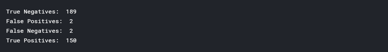
#extracting true_positives, false_positives, true_negatives, false_negatives
tn, fp, fn, tp = confusion_matrix(y_test, y_pred).ravel()
print("True Negatives: ",tn)
print("False Positives: ",fp)
print("False Negatives: ",fn)
print("True Positives: ",tp)
How Accurate is our Model?
#Accuracy
Accuracy = (tn+tp)*100/(tp+tn+fp+fn)
print("Accuracy {:0.2f}%:",.format(Accuracy))

Does Accuracy matter?
Not always, it may not be the right measure at times, especially if your Target class is not balanced (data is skewed). Then you may consider additional metrics like Precision, Recall, F score (combined metric), but before diving in lets take a step back and understand the terms that form the basis for these.
Some Basic Terms
True Positive — Label which was predicted Positive (in our scenario Authenticated Bank Notes) and is actually Positive (i.e. belong to Positive ‘Authorized’ Class).
True Negative — Label which was predicted Negative (in our scenario Forged Bank Notes) and is actually Negative (i.e. belong to Negative ‘Forged’ Class).
False Positive — Label which was predicted as Positive, but is actually Negative, or in simple words the Note wrongly predicted as Authentic by our Model, but is actually Forged. In Hypothesis Testing it is also known as Type 1 error or the incorrect rejection of Null Hypothesis, refer this to read more about Hypothesis testing.
False Negatives — Labels which was predicted as Negative, but is actually Positive (Authentic Note predicted as Forged). It is also known as Type 2 error, which leads to the failure in rejection of Null Hypothesis.
Now lets look at most common evaluation metrics every Machine Learning Practitioner should know!


Metrics beyond Accuracy
Precision
It is the ‘Exactness’, ability of the model to return only relevant instances. If your use case/problem statement involves minimizing the False Positives, i.e. in current scenario if you don’t want the Forged Notes to be labelled as Authentic by the Model then Precision is something you need.
#Precision
Precision = tp/(tp+fp)
print("Precision {:0.2f}".format(Precision))


Recall
It is the ‘Completeness’, ability of the model to identify all relevant instances, True Positive Rate, aka Sensitivity. In the current scenario if your focus is to have the least False Negatives i.e. you don’t Authentic Notes to be wrongly classified as Forged then Recall can come to your rescue.
#Recall
Recall = tp/(tp+fn)
print("Recall {:0.2f}".format(Recall))

F1 Measure
Harmonic mean of Precision & Recall, used to indicate a balance between Precision & Recall providing each equal weightage, it ranges from 0 to 1. F1 Score reaches its best value at 1 (perfect precision & recall) and worst at 0, read more here.
#F1 Score
f1 = (2*Precision*Recall)/(Precision + Recall)
print("F1 Score {:0.2f}".format(f1))

F-beta Measure
It is the general form of F measure — Beta 0.5 & 2 are usually used as measures, 0.5 indicates the Inclination towards Precision whereas 2 favors Recall giving it twice the weightage compared to precision.


#F-beta score calculation
def fbeta(precision, recall, beta):
    return ((1+pow(beta,2))*precision*recall)/(pow(beta,2)*precision + recall)

f2 = fbeta(Precision, Recall, 2)
f0_5 = fbeta(Precision, Recall, 0.5)

print("F2 {:0.2f}".format(f2))
print("\nF0.5 {:0.2f}".format(f0_5))

Specificity
It is also referred to as ‘True Negative Rate’ (Proportion of actual negatives that are correctly identified), i.e. more True Negatives the data hold the higher its Specificity.
#Specificity
Specificity = tn/(tn+fp)
print("Specificity {:0.2f}".format(Specificity))

ROC (Receiver Operating Characteristic curve)
The plot of ‘True Positive Rate’ (Sensitivity/Recall) against the ‘False Positive Rate’ (1-Specificity) at different classification thresholds.
The area under the ROC curve (AUC ) measures the entire two-dimensional area underneath the curve. It is a measure of how well a parameter can distinguish between two diagnostic groups. Often used as a measure of quality of the classification models.
A random classifier has an area under the curve of 0.5, while AUC for a perfect classifier is equal to 1.
#ROC
import scikitplot as skplt #to make things easy
y_pred_proba = LR.predict_proba(X_test)
skplt.metrics.plot_roc_curve(y_test, y_pred_proba)
plt.show()

Conclusion
Since the problem selected to illustrate the use of Confusion Matrix and related Metrics was simple, you found every value on higher level (98% or above) be it Precision, Recall or Accuracy; usually that will not be the case and you will require the domain knowledge about data to choose between the one metric or other (often times a combination of metrics).
For example: if its about finding that ‘spam in your mailbox’, high Precision of your model will be of much importance (as you don’t want the ham to be labelled as spam), it will tell us what proportion of messages we classified as spam, actually were spam. Ratio of true positives(words classified as spam, and which are actually spam) to all positives(all words classified as spam, irrespective of whether that was the correct classification). While in Fraud detection you may wish your Recall to be higher, so that you can correctly classify/identify the Frauds even if you miss classify some of the non-fraudulent activity as Fraud, it won’t cause any significant damage.
Source: https://towardsdatascience.com/demystifying-confusion-matrix-confusion-9e82201592fd


Comments
Post a Comment