K-Nearest Neighbors in Python + Hyperparameters Tuning
“The k-nearest neighbors algorithm (KNN) is a non-parametric method used for classification and regression. In both cases, the input consists of the k closest training examples in the feature space. The output depends on whether k-NN is used for classification or regression”-Wikipedia
So actually KNN can be used for Classification or Regression problem, but in general, KNN is used for Classification Problems. Some applications of KNN are in Handwriting Recognition, Satellite Image Recognition, and ECG Pattern Recognition. This algorithm is very simple but is often used by Data Scientists.
In Overview, the KNN algorithm works to classify new data based on its proximity to K-neighbors (training data). So if the new data is surrounded by training data that has Class 1, it can be concluded that the new data is included in Class 1. To make it easier to understand, see the illustration below.

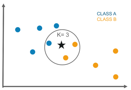
The picture above wants to classify new data with the star symbol, if You choose K = 3, then 3 closest data will be searched to the star data. After that, you inspect these 3 data classes. If you see from Figure, the 3 closest data are 2 in Class B and 1 in Class A, so it can be said that star data is included in Class B. In more detail, how KNN works is as follows:
1. Determine the value of K.
The first step is to determine the value of K. The determination of the K value varies greatly depending on the case. If using the Scikit-Learn Library the default value of K is 5.
2. Calculate the distance of new data with training data.
To calculate distances, 3 distance metrics that are often used are Euclidean Distance, Manhattan Distance, and Minkowski Distance.

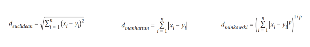
When you use Scikit-Learn, the default distance used is Euclidean. It can be seen in the Minkowski distance formula that there is a Hyperparameter p, if set p = 1 then it will use the Manhattan distance and p = 2 to be Euclidean.
3. Find the closest K-neighbors from the new data.
After calculating the distance, then look for K-Neighbors that are closest to the new data. If using K = 3, look for 3 training data that is closest to the new data.
4. New Data Class Prediction.
To determine the class of new data, select the class of training data that closest to the new data and have the highest quantity.
5. Evaluation.
Calculate the accuracy of the model, if the accuracy is still low, then this process can be repeated again from step 1.
After knowing how KNN works, the next step is implemented in Python. I will use Python Scikit-Learn Library. The dataset I will use is a heart dataset in which this dataset contains characteristics of the patient whether the patient has heart disease or not.
To follow this tutorial, you should at least know about:
1. Basic programming in Python.
2. Pandas and Numpy libraries for data analysis tools.
3. Matplotlib and Seaborn libraries for data visualization.
4. Scikit-Learn Library for Machine Learning.
5. Jupyter Notebook.
The steps in solving the Classification Problem using KNN are as follows:
1. Load the library
2. Load the dataset
3. Sneak peak data
4. Handling missing values
5. Exploratory Data Analysis (EDA)
6. Modeling
7. Tuning Hyperparameters
Dataset and Full code can be downloaded at my Github and all work is done on Jupyter Notebook.
1Loading several libraries that will be used to do the analysis in this tutorial. I assume that you have already installed the library.
import pandas as pd
import numpy as npimport matplotlib.pyplot as plt
import seaborn as snsfrom sklearn.neighbors import KNeighborsClassifier
from sklearn.metrics import classification_report
from sklearn.model_selection import train_test_split
from sklearn.metrics import roc_auc_score
from sklearn.model_selection import GridSearchCV
2Load the dataset to be used, dataset contains historical data from patients who have been examined for heart disease.
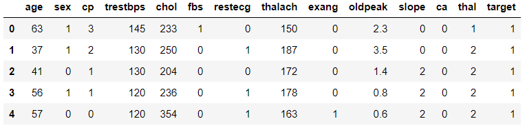
df = pd.read_csv('heart.csv')3Let’s see some general information from the data to be more familiar with our data.
df.head()
df.shape

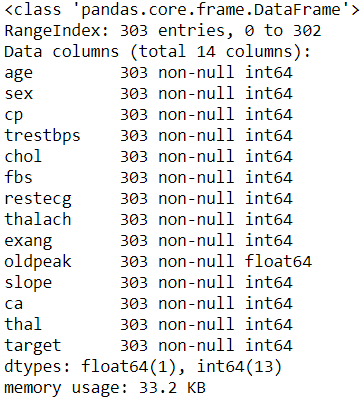
df.info()
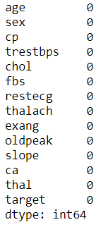
4Checking whether there is missing data or not, if not then it can proceed to the Exploratory Data Analysis (EDA) stage.
df.isnull().sum()
5Conducting Exploratory Data Analysis (EDA) to understand our data better (only a few are displayed, complete on Github).
#Univariate analysis target.
sns.countplot(df['target'])
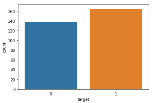
- Looks like the target feature is balanced because the number of values 0 and 1 does not differ much.
- Value 0 for Heart Disease.
- Value 1 for No Heart Disease.
#Univariate analysis age.
f = plt.figure(figsize=(20,4))
f.add_subplot(1,2,1)
sns.distplot(df['age'])
f.add_subplot(1,2,2)
sns.boxplot(df['age'])
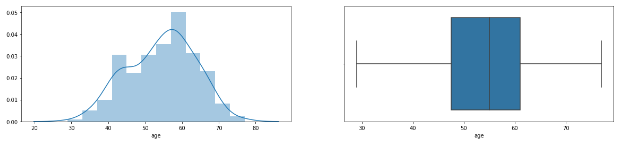
- From the distplot, it can be seen that the density of the data lies in the range of 50–60 years and very rarely patients aged 30 years or below or 80 years and above.
- The boxplot shows that the data has no outliers.
#Univariate analysis sex: 1=male; 0=female.
#Univariate analysis chest pain type (cp): 0=typical angina; 1=atypical angine; 2=non-anginal pain; 3=asymptomatic
#Univariate analysis fasting blood sugar: 1 if > 120 mg/dl; 0 otherwise.f = plt.figure(figsize=(20,4))
f.add_subplot(1,3,1)
df['sex'].value_counts().plot('bar', color='red')
f.add_subplot(1,3,2)
df['cp'].value_counts().plot('bar', color='green')
f.add_subplot(1,3,3)
sns.countplot(df['fbs'], color='yellow')

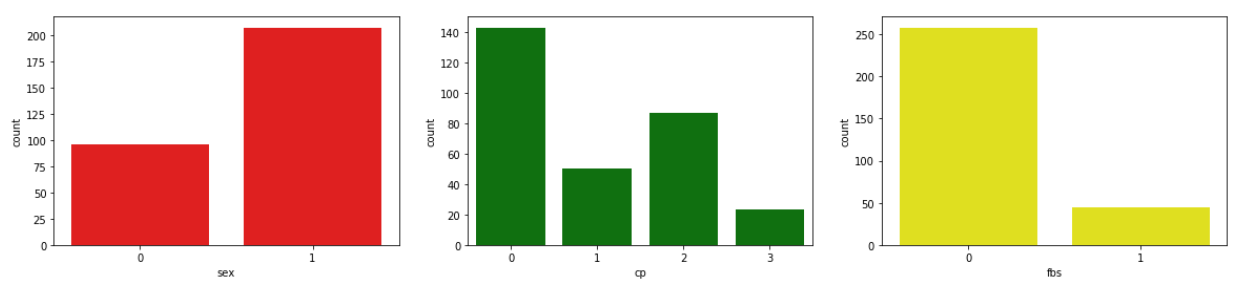
- Male patients turns out to have more numbers or even 2 times the number of female patients.
- Most patients have type CP 0, which is typical angine and the least type is 3, which is asymptomatic.
- The plot above shows that there are many fasting blood sugar values below 120 or 0.
#Univariate analysis resting blood pressure (mm Hg) atau trestbps.f = plt.figure(figsize=(20,4))
f.add_subplot(1,2,1)
sns.distplot(df['trestbps'])
f.add_subplot(1,2,2)
sns.boxplot(df['trestbps'])

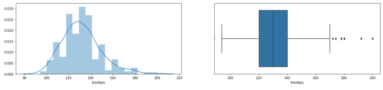
- For the value of resting blood pressure or trestbps, the most numbers are ranged from 120 to 140 mmHg.
- The trestbps feature has several outliers.
6The next stage is to make a model that will be used to predict patients. In this case, we will use KNN algorithm.
#Create KNN Object.
knn = KNeighborsClassifier()#Create x and y variables.
x = df.drop(columns=['target'])
y = df['target']#Split data into training and testing.
x_train, x_test, y_train, y_test = train_test_split(x, y, test_size=0.2, random_state=4)#Training the model.
knn.fit(x_train, y_train)#Predict test data set.
y_pred = log_reg.predict(x_test)#Checking performance our model with classification report.
print(classification_report(y_test, y_pred))#Checking performance our model with ROC Score.
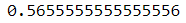
roc_auc_score(y_test, y_pred)

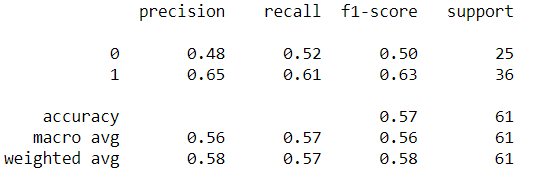

- From the classification report, it can be seen that the model has an average performance of around 57% ranging from precision, recall, f1-score, and support. Accuracy also shows in value of 57%.
- Then for the AUC score, it can be seen that the value is around 56.5%.
7Because the performance is still low, Let's try to use Hyperparameter Tuning to Improve Model Performance.
#List Hyperparameters that we want to tune.
leaf_size = list(range(1,50))
n_neighbors = list(range(1,30))
p=[1,2]#Convert to dictionary
hyperparameters = dict(leaf_size=leaf_size, n_neighbors=n_neighbors, p=p)#Create new KNN object
knn_2 = KNeighborsClassifier()#Use GridSearch
clf = GridSearchCV(knn_2, hyperparameters, cv=10)#Fit the model
best_model = clf.fit(x,y)#Print The value of best Hyperparameters
print('Best leaf_size:', best_model.best_estimator_.get_params()['leaf_size'])
print('Best p:', best_model.best_estimator_.get_params()['p'])
print('Best n_neighbors:', best_model.best_estimator_.get_params()['n_neighbors'])

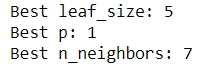
- From GridSearch, it can be seen that the best number of leaf_size is 5 while the optimal distance method is Manhattan or p = 1.
- Then the most optimal number of K is 7.

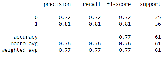

- Using Hyperparameters Tuning can improve model performance by about 20% to a range of 77% for all evaluation matrices.
- The ROC value also increased to 76%.
But even though the performance has improved at 77%, I am not sure about my model and will make some modifications that I will share next week. One of the things I will do is rescaling using StandardScalar.
Thank you for reading this story until the end, if there are criticisms or suggestions you can immediately comment and if the story is useful you can clap or share it!
https://medium.com/datadriveninvestor/k-nearest-neighbors-in-python-hyperparameters-tuning-716734bc557f


Comments
Post a Comment