train_test_split Vs StratifiedShuffleSplit

 In a just concluded Kaggle competition i participated in, i used both types of split approaches without really having the intuition of why i choose one over the other. In real life you wouldn’t want to be performing trial and error as it might be costly in both resources and time. So this article will give you a better understanding of what is, when to and why to use these two distinctive splits as you make efforts to be a better data scientist. Before we talk about the two kinds of data splits, lets firstly answer some quick questions that have roots in explaining this topic. Some of the quick questions to answer are:

• What is sampling?
• What is sampling bias?

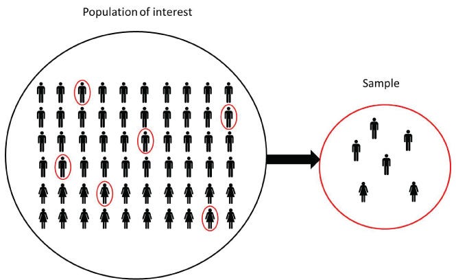
What is sampling?

Sampling is the selection of s subset of individuals from with a statistical population to estimate characteristics of the whole population. Studying the whole may be exhaustive, so taking a part that represent the whole and study it is way realistic, and that is the point of sampling. An illustration of the sample and population can be seen below.

An Illustration of Population and Sample

What is Sampling Bias?

This happens when a sample is collected in such a way that some members of the intended population have a lower sampling probability (i.e the probability of becoming part of the sample during drawing of a single sample) than others. This results in the sample collected favoring a particular group from the population, making it likely for some groups not being selected (thereby leaving an important part out of study).

Photo by Alex on Unsplash

So back to how we split our data sets…

Splitting our data sets into training sets and test set can be done under the two sampling techniques

1. Random Sampling: This is a sampling technique in which a subset of a statistical population is taken out, where each member of the population has an equal opportunity of being selected. For example, imagine we have a 1000 dogs and we want to take a sample of 200 dogs. In this process each of the 3000 dogs has an equal opportunity(probability) of being selected in the 200 dogs needed in the sample. Random sampling is ideal when there is not much information about a population or when the data is diverse and not easily grouped.
2. Stratified Sampling: This is a sampling technique that is best used when a statistical population can easily be broken down into distinctive sub-groups. Then samples are taken from each sub-groups based on the ratio of the sub groups size to the total population. Using the dogs example again, imagine now we have four distinctive breed of dogs in the 1000 population broken down into A:450, B:250, C:200 and D:100. To perform the sampling of the 200 dogs needed, 45% of the sample must come from A, 25% from B, 20% from C and lastly 10% must come from D. Using Stratified Sampling technique ensures that there will be selection from each sub-groups and prevents the chance of omitting one sub-group leading to sampling bias thus making the dog population happy!

Photo by anya potsiadlo on Unsplash

During data splitting operations, train_test_split represents random sampling while StratifiedShuffleSplit represents Stratified Sampling. So lets illustrate how to use these techniques in codes (in python). In will be using the California data sets to explain these concepts, both the data and my notebook can be found HERE.

So we start by importing important relevant libraries we need to start the project and read in the California housing data

Next, we would to view what the descriptive statistics of the data sets are, this can be done via

It is good practice to visualize the data sets, to see what you are working with, this can be done as follows

Using the correlation heatmap to visualize and observe features and target correlations.

It can be observed from the heatmap that median_income is highly correlated to the target, having ‘0.69’, so lets look at the feature more closely. we have seen from the correlation heatmap that the ‘median_income’ feature is important. We will want our test set to be representative of the various categories of income in the whole dataset. If we look at the histogram of the ‘median_income’ we created before, you will observe that that most of median income values are clustered around 1.5 t0 7 (i.e $15,000-$70,000), but some ‘median_income’ values go far beyond 7.

Now lets see how both approaches are impemented! The moment we have been waiting for😀, lets move🚀

Firstly the random sampling approach (i.e train_test_split), using a test size of 30% of data and a random_state of 42. The random_state is a what you use to prevent snooping the entire data sets, as it ensures you always generate the same shuffled indices, it can have various values but most people chose 42 since in has a unique universal importance, you could read about those Here.

Next to the Stratified Sampling approach (i.e StratifiedShuffleSplit).Since it has been observed that the 'median_income' feature is important. We will want our test set to be representative of the various categories of income in the whole dataset. If we look at the histogram of the 'median_income' we created before, you will observe that that most of median income values are clustered around 1.5 t0 7 (i.e $15,000-$70,000), but some 'median_income' values go far beyond 7.

N/B: It is important to have a sufficient number of instances in your data sets for each stratum, or else the estimate of the stratum's importance may be biased. This means that you shouldn't have too much strata, and each stratum should be large enough.

So 5 strata were created in this project.We will create 5 category attribute labeled 1 to 5(where label 1 depicts values from 0-2,label 2 depicts values from 2-4 an so on till label 5 depicts 8-inf which covers the remaining values on the histogram)

We can observe the proportion of the split as compared with the ‘income_cat’ histogram. it is observed that the data were split in accordance to the strata in the ‘income_cat’ histogram.

We can evaluate both approaches via the snippet below, as you can test sets generated using the stratified approach (stratified sample) are similar to the overall dataset (population), whereas the test set generated using purely random sampling is quite skewed.

In summary we had 14448 rows and 10 columns (14448, 10) and 6192 rows and 10 columns (6192, 10) for the train and test set respectively for both approaches with the two different sampling techniques.

https://medium.com/@411.codebrain/train-test-split-vs-stratifiedshufflesplit-374c3dbdcc36