Evaluation metrics in classification algorithms
This blog is completely dedicated to the crucial metrics used in classification problems. You might have come across problem statements where we have to use metrics other than the well known ‘accuracy’ score. Let us try to understand confusion matrix, accuracy, recall, precision, F1 Score, ROC- AUC curve and their usage.

Accuracy score is widely used for evaluating model which do not have any issue with type I and II errors or if it is a balanced data set. But certain problems like cancer analysis or customer churn data which are imbalanced, the focus will mainly be on False Positives and False Negatives. In such situations, we need other metrics — Recall, Precision and F1-Score. Recall is the measure of actual true values captured by the model where as Precision is the measure of relevant true values predicted by the model. F1-Score is the harmonic mean of recall and precision. All of them ranges from 0 — 1 and any score close to 1 is considered good. This might be confusing a bit. Lets understand in detail with an example.
Here is a problem statement where we have to predict if a tumor is benign or malignant based on few features. I have used logistic regression for modelling in the previous blog and the results are as following:

Analysing the confusion matrix of train data, by comparing to fig.1 above.
TN = 240, TP = 130, FP = 19, FN = 9.
Accuracy =(240+130)/(240+130+19+9)= 0.93 i.e., 93% of the predictions are correctly classified
Recall = 130/(130+9) =0.93 i.e., Model correctly identifies 93% of all malignant tumors
Precision = 130/(130+19) = 0.87 i.e., the model is correct 87% of the time in classifying malign(out of 149 predicted true values, 130 are correct)
F1- Score = 2*0.87*0.93/(0.87+0.93) = 0.89
If we would have had precision and F1-Scores less than 0.5 then we should try out models other than logistic regression for classification. As we have pretty good scores of above 0.85, we can treat this model is fairly good but we should always try to increase F1-Score to avoid wrong predictions of Malign and Benign.
Trade off of Recall and Precision.
In logistic regression, while classifying into Malign or Benign, there is a threshold value of the probability which is 0.5 by default. If the probability function results in p≥0.5 then it is Malign else Benign. But if the threshold moves below or above 0.5 then all the metrics will change. This results in a trade off between Recall and Precision.
In the tumor problem, we do not want to have False Negatives(type II errors) i.e., predicting a tumor is Benign though in reality it is Malignant. So we choose a model that can perform this task of reducing FNs that in turn increases the score of Recall. But due to this threshold changing, FP’s will increase, leading to low Precision. This is called Recall Precision Tradeoff.
ROC — AUC:
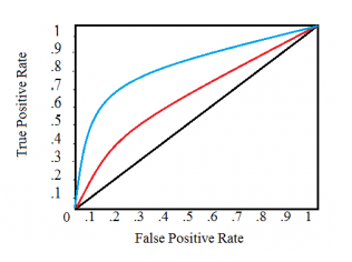
Receiver operating characteristics: An evaluation metric where we can visualize the performance of the model is called ROC curve. This is plotted on True Positive rate against False Positive rates for different threshold values (probabilities as explained above). This optimal threshold helps in achieving Precision Recall balance.

The black line shows the rates for a random classifier. Red and blue curves are for different models. We can have only one curve for one model. At different thresholds, the function for ROC plots this graph. At a threshold of 1, there are no positives and negatives yet so the graph starts from 0 and as threshold increases, the curve moves towards right upwards as more TP and FP’s come into picture.
We can quantify the performance of the model using this curve by finding the area under the curve — AUC (using differentials but the package takes care of it all). AUC values ranges from 0–1, any score near 1 evaluates as a good model.
Hope this helps in understanding the important metrics used for classification. Happy learning! :)


Comments
Post a Comment