The ultimate practical guide to understand, spot, clean, impute missing data — Benchmark of strategies on a real-world example.

Throughout this article, you will become good at spotting, understanding, and imputing missing data. We demonstrate various imputation techniques on a real-world logistic regression task using Python. Properly handling missing data has an improving effect on inferences and predictions. This is not to be ignored.

The first part of this article presents the framework for understanding missing data. Later we demonstrate the most popular strategies in dealing with missingness on a classification task to predict the onset of diabetes.

Missing data is hard to avoid

A considerable part of data science or machine learning job is data cleaning. Often when data is collected, there are some missing values appearing in the dataset.

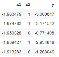
To understand the reason why data goes missing, let’s simulate a dataset with two predictors x1, x2, and a response variable y.

We will virtually make some data missing to illustrate various reasons why many real-world datasets may contain missing values.

There are 3 major types of missing values to be concerned about.

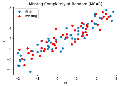
Missing Completely at Random (MCAR)

MCAR occurs when the probability of missing values in a variable is the same for all samples.

For example, when a survey is conducted, and values were just randomly missed when being entered in the computer or a respondent chose not to respond to a question.

There is no effect of MCAR on inferences made by a model trained on such data.

To illustrate MCAR, we randomly remove half of the values for x1 as follows.

## Missing Completely at Random (MCAR)

	# randomly mark half of x1 samples as missing MCAR
	# independend of any information recorded
	idx_mcar= np.random.choice([0, 1], size=(100,)) == 1

	plt.scatter(x1,y, label='data')
	plt.scatter(x1[idx_mcar],y[idx_mcar], label='missing (MCAR)', color='red')
	plt.xlabel('x1')
	plt.ylabel('y')
	plt.legend()
	plt.title('Missing Completely at Random (MCAR)');

Missing at Random (MAR)

The probability of missing values, at random, in a variable depends only on the available information in other predictors.

For example, when men and women respond to the question “have you ever taken parental leave?”, men would tend to ignore the question at a different rate compared to women.

MARs are handled by using the information in the other predictors to build a model and impute a value for the missing entry.

We simulate MAR by removing x1 values depending on x2 values. When x2 has the value 1, then the corresponding x1 is missing.

## Missing at Random (MAR)

	# randomly mark half of x1 samples as missing MAR
	# depending on value of recorded predictor x2

	idx_mar = x2 == 1

	fig, ax = plt.subplots(1,2,figsize=(15,5))
	ax[0].scatter(x1, y, label='data')
	ax[0].scatter(x1[idx_mar], y[idx_mar], label='missing', color='red')
	ax[0].set_xlabel('x1')
	ax[0].set_ylabel('y')
	ax[0].legend()
	ax[0].set_title('Missing at Random (MAR)');
	ax[1].vlines(x1[x2 == 1], 0, 1, color='black')
	ax[1].set_xlabel('x1')
	ax[1].set_ylabel('x2')
	ax[1].set_title('dependent predictor - measured');

Missing Not at Random (MNAR)

The probability of missing values, not at random, depends on information that has not been recorded, and this information also predicts the missing values.

For example, in a survey, cheaters are less likely to respond when asked if they have ever cheated.

MNARs are almost impossible to handle.

Luckily there shouldn’t be any effect of MNAR on inferences made by a model trained on such data.

Assuming that there is a hypothetical variable x3 that was not measured, but determines which x1 values are missing, we can simulate MNAR as follows.

## Missing Not at Random (MNAR)

	# randomly mark half of x1 samples as missing MNAR
	# depending on unrecorded predictor x3
	x3 = np.random.uniform(0, 1, 100)
	idx_mnar = x3 > .5

	fig, ax = plt.subplots(1,2,figsize=(15,5))
	ax[0].scatter(x1, y, label='data')
	ax[0].scatter(x1[idx_mnar], y[idx_mnar], label='missing', color='red')
	ax[0].set_xlabel('x1')
	ax[0].set_ylabel('y')
	ax[0].legend()
	ax[0].set_title('Missing Not at Random (MNAR)');
	ax[1].scatter(x1, x3, color='black')
	ax[1].axhline(.5, -3, 3)
	ax[1].set_xlabel('x1')
	ax[1].set_ylabel('x3')
	ax[1].set_title('dependent predictor - not measured');

3 Main Approaches to Compensate for Missing Values

It generally cannot be determined whether data are missing at random, or whether the missingness depends on unobserved predictors or the missing data themselves.

In practice, the missing at random assumption is reasonable.

Several different approaches to imputing missing values are found in the literature:

1. Imputation using zero, mean, median or most frequent value

This works by imputing all missing values with zero, the mean or median for quantitative variables, or the most common value for categorical variables.

Additionally, we can create a new variable that is an indicator of missingness and includes it in the model to predict the response. This is done after plugging in zero, mean, median, or most frequent value in the actual variable.

2. Imputation using a randomly selected value

This works by randomly selecting an observed entry in the variable and use it to impute missing values.

3. Imputation with a model

This works by replacing missing values with predicted values from a model based on the other observed predictors.

The k nearest neighbor algorithm is often used to impute a missing value based on how closely it resembles the points in the training set.

Model-based imputation with uncertainty works by replacing missing values with predicted values plus randomness from a model based on the other observed predictors.

Model-based progressive imputation uses previously imputed missing values to predict other missing values.

Additional methods include Stochastic Regression Imputation, Multiple Imputations, Datawig, Hot-Deck imputation, Extrapolation, Interpolation, Listwise Deletion.

A Practical Guide for Handling Missing Values

Describing the data

In the following sections, we are going to use the Pima Indians onset of diabetes dataset to be found here.

This dataset describes patient medical record data for Pima Indians and whether they had an onset of diabetes within five years.

It is a binary classification problem (onset of diabetes as 1 or not as 0).

The input variables that describe each patient are numerical and have varying scales.

The list below shows the eight attributes plus the target variable for the dataset:

The number of times the patient was pregnant.
2-hours plasma glucose concentration per 2 hours in an oral glucose tolerance test.
Diastolic blood pressure (mm Hg).
Triceps skinfold thickness (mm).
2-hours serum insulin (mu U/ml).
Body mass index.
Diabetes pedigree function.
Age (years).
Outcome (1 for early onset of diabetes within five years, 0 for not).

import pandas as pd

	pima_df = pd.read_csv('pima-indians-diabetes.csv')

	response = 'Outcome'
	predictors = pima_df.columns.difference([response]).values

	pima_df.describe()

The data has 764 observations and 9 features. We immediately see strange values for some of the predictors.

Pregnancies range up to 17. The blood pressure, glucose, skin thickness, insulin, and BMI variables include zeros, which are physically implausible.

We will have to handle these somehow.

Properly flagging missing values

Although missing values are usually coded using NaN, Null, or None, it seems that none of the observations are marked in this way.

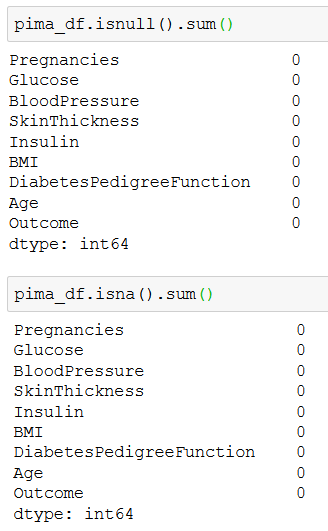
As a first step we should properly flag missing values.

In terms of missing data, the variables we need to look at most closely are Glucose, BloodPressure, SkinThickness, Insulin, and BMI, all of which contain 0 among their observations.

A quick search in the literature shows that these features cannot have a physiological value of zero. The most plausible explanation is that missing observations for features were missing were somehow replaced with zero.

This disguised missing data would mislead our later classification attempts. We will clean the data by marking disguised missing values clearly as NaN.

The response variable, which should be coded as 0 or 1, contained values with \ or } appended to the 0’s and 1s. It looks like an error similar to those introduced when reading from or writing CSVs have found their way into the data. The solution we choose is simply to remove the characters.

Looking at the data types, predictors are stored as float and the response as an object. The float data type makes sense for BMI and DiabetesPedigreeFunction. The remaining features can be stored as integers.

The following function cleans the data and replaces zeros with NaNs for the five columns discussed: Glucose, BloodPressure, SkinThickness, Insulin, and BMI.

def clean_data(df_raw,
	cols_with_zeros=['Glucose', 'BloodPressure', 'SkinThickness', 'Insulin', 'BMI'],
	response = ['Outcome']):
	df = df_raw.copy()
	# replace zero with NaN in features
	df[cols_with_zeros] = df[cols_with_zeros].replace(0, np.nan)
	# remove \ and } from response
	df = df.replace(to_replace=r'\\\|\}', value='', regex=True)
	# change response data type to int
	df[response] = df[response].astype('int')
	return df

	pima_df_cleaned = clean_data(pima_df)
	pima_df_cleaned.head()

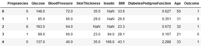
We have replaced any zero and indicated missing values with NaN.

Exploring missing values

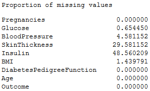
We can now calculate the proportion of missing values for each feature: 48.56% of Insulin, 29.58% of SkinThickness, 4.58% of BloodPressure, 1.43% of BMI, and 0.65% of Glucose. The remaining features do not have any missing values.

	print("Proportion of missing values")
	missing_values_count = pima_df_cleaned.isna().sum()*100/pima_df_cleaned.shape[0]
	features_with_missing_values = missing_values_count[missing_values_count>0].index.values
	missing_values_count

As a second step, we might need to perform some statistical tests of the hypothesis that the features are Missing at Random (MAR), Missing Completely at Random (MCAR), or Missing not at Random (MNAR).

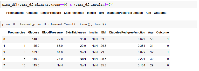
By looking closer, it seems that missing values for SkinThickness are correlated with missing values for Insulin. When SkinThickness is missing, then Insulin is also missing.

Furthermore, when BloodPressure or BMI is missing, then the probability is higher that Insulin or SkinThickness values will be missing as well.

As a third step, we explore and choose the most appropriate technique to handle missing values.

Strategies for handling missing data

We move on by providing a Python function where the following data imputation strategies are implemented.

The drop strategy removes all observations where at least one of the features has a missing value (NaN).

The mean strategy replaces any missing value (NaN) by the mean of all values available for that feature.

The median strategy and most-frequent strategy replace missing values by the median or the most frequently appearing values, respectively.

The model-based strategy uses the features without missing values for training kNN regression models.

We choose kNN in order to capture the variability of available data. This would not be the case if we would use a linear regression model that would predict missing values along a regression line.

We distinguish between two modes in this model-based strategy. The following features are used as predictors in the basic mode: Age, DiabetesPedigreeFunction, Outcome, Pregnancies. The fitted model is used to predict the missing values in the remaining features.

In the progressive mode, after we fill in missing values in a given feature, we consider the feature as a predictor for estimating the missing values of the next feature.

The imputed data can be optionally standardized between 0 and 1. This might improve the performance of classification using regularized logistic regression.

Because the features are on a different scale (e.g., Age vs. Insulin) and their values range differs (e.g., Pedigree vs. Insulin), the shrinkage penalty could be wrongly calculated if features are not scaled.

from sklearn.impute import SimpleImputer
	from sklearn.neighbors import KNeighborsRegressor
	from sklearn.preprocessing import MinMaxScaler

	# function for KNN model-based imputation of missing values using features without NaN as predictors
	def impute_model_basic(df):
	cols_nan = df.columns[df.isna().any()].tolist()
	cols_no_nan = df.columns.difference(cols_nan).values
	for col in cols_nan:
	test_data = df[df[col].isna()]
	train_data = df.dropna()
	knr = KNeighborsRegressor(n_neighbors=5).fit(train_data[cols_no_nan], train_data[col])
	df.loc[df[col].isna(), col] = knr.predict(test_data[cols_no_nan])
	return df

	# function for KNN model-based imputation of missing values using features without NaN as predictors,
	# including progressively added imputed features
	def impute_model_progressive(df):
	cols_nan = df.columns[df.isna().any()].tolist()
	cols_no_nan = df.columns.difference(cols_nan).values
	while len(cols_nan)>0:
	col = cols_nan[0]
	test_data = df[df[col].isna()]
	train_data = df.dropna()
	knr = KNeighborsRegressor(n_neighbors=5).fit(train_data[cols_no_nan], train_data[col])
	df.loc[df[col].isna(), col] = knr.predict(test_data[cols_no_nan])
	cols_nan = df.columns[df.isna().any()].tolist()
	cols_no_nan = df.columns.difference(cols_nan).values
	return df

	# function for imputing missing data according to a given impute_strategy:
	# drop_rows: drop all rows with one or more missing values
	# drop_cols: drop columns with one or more missing values
	# model_basic: KNN-model-based imputation with fixed predictors
	# model_progressive: KNN-model-based imputation with progressively added predictors
	# mean, median, most_frequent: imputation with mean, median or most frequent values
	#
	# cols_to_standardize: if provided, the specified columns are scaled between 0 and 1, after imputation
	def impute_data(df_cleaned, impute_strategy=None, cols_to_standardize=None):
	df = df_cleaned.copy()
	if impute_strategy == 'drop_rows':
	df = df.dropna(axis=0)
	elif impute_strategy == 'drop_cols':
	df = df.dropna(axis=1)
	elif impute_strategy == 'model_basic':
	df = impute_model_basic(df)
	elif impute_strategy == 'model_progressive':
	df = impute_model_progressive(df)
	else:
	arr = SimpleImputer(missing_values=np.nan,strategy=impute_strategy).fit(
	df.values).transform(df.values)
	df = pd.DataFrame(data=arr, index=df.index.values, columns=df.columns.values)
	if cols_to_standardize != None:
	cols_to_standardize = list(set(cols_to_standardize) & set(df.columns.values))
	df[cols_to_standardize] = df[cols_to_standardize].astype('float')
	df[cols_to_standardize] = pd.DataFrame(data=MinMaxScaler().fit(
	df[cols_to_standardize]).transform(df[cols_to_standardize]),
	index=df[cols_to_standardize].index.values,
	columns=df[cols_to_standardize].columns.values)
	return df

Logistic regression with missing data

In this section, we fit a logistic regression model on the cleaned data after applying a specific imputation strategy:

dropping rows with missing values,
dropping columns with missing values,
imputing missing values with column mean,
imputing missing values with model-based prediction,

imputing missing values with progressive model-based prediction.

from sklearn.model_selection import train_test_split
	from sklearn.linear_model import LogisticRegressionCV
	from sklearn.metrics import accuracy_score
	from timeit import default_timer as timer

	# function for handling missing values
	# and fitting logistic regression on clean data
	def logistic_regression(data, impute_strategy=None,
	cols_to_standardize=None,
	test_size=0.25,
	random_state=9001):
	start = timer()

	# store original columns
	original_columns = data.columns.difference(['Outcome'])
	df_imputed = impute_data(data, impute_strategy, cols_to_standardize)
	train_data, test_data = train_test_split(df_imputed, test_size=test_size,
	random_state=random_state)

	# note which predictor columns were dropped or kept
	kept_columns = df_imputed.columns.difference(['Outcome'])
	dropped_columns = original_columns.difference(df_imputed.columns)
	original_columns = original_columns.difference(['Outcome'])

	# prepare tensors
	X_train = train_data.drop(columns=['Outcome'])
	y_train = train_data['Outcome']
	X_test = test_data.drop(columns=['Outcome'])
	y_test = test_data['Outcome']

	# model training
	logistic_model = LogisticRegressionCV(cv=10, penalty='l2', max_iter=1000).fit(
	X_train, y_train)

	# model evaluation
	train_score = accuracy_score(y_train, logistic_model.predict(X_train))
	test_score = accuracy_score(y_test, logistic_model.predict(X_test))
	duration = timer() - start
	print("Classification rate on training data: {}".format(train_score))
	print("Classification rate on test data: {}".format(test_score))
	print("Execution time: {}".format(duration))

	return {
	'imputation strategy': impute_strategy,
	'standardized': cols_to_standardize!=None,
	'model': logistic_model,
	'train score': train_score,
	'test score': test_score,
	'execution time (s)': duration
	}

	# list to store models' performance
	lr_results = []

	# prepare data
	pima_df_cleaned = clean_data(pima_df)
	cols_to_standardize=['Age','BMI','BloodPressure','Glucose','Insulin','Pregnancies','SkinThickness','DiabetesPedigreeFunction']

	# fit logistic regression for each imputation strategy
	# with and without standardizing features
	for impute_strategy in ['drop_rows', 'mean', 'model_basic', 'model_progressive']:
	for cols in [None, cols_to_standardize]:
	result = logistic_regression(pima_df_cleaned, impute_strategy=impute_strategy, cols_to_standardize=cols)
	lr_results.append(result)

	# display logistic regression performance
	lr_results_df = pd.DataFrame(lr_results)
	lr_results_df.drop(['model'], axis=1).drop_duplicates()

It is worth noticing the significant effect that imputation brings to the values of estimated parameters and their accuracy.

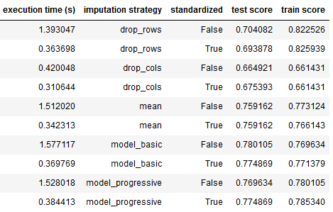
Effect of dropping strategy on accuracy

By dropping rows or columns with missing values, we lose valuable information that might have a significant impact on the response variable.

The consequence is overfitting in the training dataset and worse prediction performance on the test dataset.

Effect of mean/model imputation on accuracy

The mean imputation of missing data reduces overfitting and improves the prediction on the test dataset.

Classification is the best when a model-based is used when imputing missing data. This is because the original variance of the data is better approached when using k-nearest neighbors as a replacement of missing data.

Effect of imputation on training time

The computational complexity is assessed by measuring the cumulative execution time of imputation, logistic regression model fitting, and prediction.

The execution time for the model-based approach is the highest when predictors are not standardized. Calculating the euclidian distance to nearest neighbors requires more execution time than calculating the mean of data.

When dealing with a very large number of observations, we might prefer mean imputation at the cost of lower classification accuracy.

Effect of imputation on inference

We retrieve the coefficients estimated by our regularized logistic regression models as follows.

# get index of strategies
	lr_results_df = pd.DataFrame(lr_results)
	strategies = lr_results_df['imputation strategy']

	# get a boolean array where True => standardized
	standardized = lr_results_df['standardized']
	st = lambda s: ' standardized' if s else ''
	coefs_ = {}
	for key, value in enumerate(strategies):
	if value == 'drop_cols':
	# skip
	pass
	else:
	strategy = value + st(standardized[key])
	coefs_[strategy] = lr_results_df['model'][key].coef_[0]
	coef_df = pd.DataFrame(data=coefs_, index=predictors)
	coef_df.T

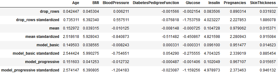
The coefficients in the table show how each predictor affects the likelihood of diabetes occurrence.

Positive values indicate factors in favor of the onset of diabetes.

Values around zero suggest that the associated predictors do not contribute much to diabetes onset.

The table shows inferred coefficients after applying an imputation strategy for missing data. Coefficients are also provided as obtained by logistic regression fit on standardized predictors values (after imputation).

Overall standardized coefficients are larger.
When rows/columns are dropped, the coefficient estimates change drastically, compared to their values when missing data is imputed by mean or model.
Coefficients for Insulin do not vary much between imputation methods. Insulin had the highest percentage of missing values between all predictors. This suggests that Insulin might be Missing Completely At Random (MCAR).

The following table compares the effect of mean imputation and model-based imputation on the coefficient magnitude obtained after dropping rows with missing data.

	coef_perc_df = coef_df.copy()
	cols = coef_df.columns.difference(['drop_rows']).values
	for col in cols:
	coef_perc_df[col] = np.round(100*(coef_df[col]/coef_df['drop_rows']-1))
	coef_perc_df[['drop_rows','mean','model_basic','model_progressive']]

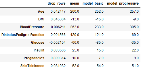
The first column shows the coefficient estimates for the logistic model trained on data where rows with missing values where removed.

The other columns show the percentage change of coefficients values after imputing missing values, compared to the drop strategy.

Age, blood pressure, and Pedigree function have the highest percentage change between dropping rows and mean/model-based imputations.

The dropping strategy is usually not the golden way.

Conclusion

In this article, we demonstrated how cleaning data and handling missing values would mean much better performance of Machine Learning algorithms.

Differentiating between MCAR, MAR, MNAR types of missing data is essential because they can affect inferences and predictions significantly.

Although there is no perfect way to handle missing data, you should be aware of the different methods available.

Compensating missing data and capitalizing on insights gained from them is one of the time-consuming parts of a Data Scientist’s job.

A model for self-driving cars that has learned from an insufficiently diverse training set is an interesting example. If the car is unsure where there is a pedestrian on the road, we would expect it to let the driver take charge. I discuss uncertainty in deep learning caused by missing data in my article below.

https://medium.com/towards-artificial-intelligence/handling-missing-data-for-advanced-machine-learning-b6eb89050357

Search This Blog

Artificial Intelligence

Handling Missing Data for Advanced Machine Learning